Seeps located adjacent to streams or rivers maintain coldwater habitats for trout and salmon during summer months when warmer water can result in fish mortality. These same sites also foster fish survival in the winter by creating a warmer environment than would normally occur. Trout and salmon abundance is related to seeps and groundwater upwelling in streams and rivers. Therefore, when pumping near a stream, we are interested not only in the resulting drawdowns, but also in the depletion of the stream flow, resulting in potentially adverse impact of groundwater dependent ecosystems.

Presented next is the first analytical model that can be used quantify stream depletion dynamics, in the special case that the aquifer is homogeneous and infinite, the stream is straight, flow is predominantly horizontal, pumping is constant, and the stream and aquifer are perfectly connected:
where:
- a =
perpendicular distance between well and stream [L]
- t =
time since pumping began [T]
- T =
aquifer transmissivity (K*thickness) [L2/T]
- S =
aquifer storage coefficient [dimensionless]
- Q =
pumping rate [L3/T]
- erfc =
the complimentary error function [dimensionless]
Develop a more general MAGNET numerical model that can reproduce the above analytical solution and perform a sensitivity analysis of stream depletion with respect to the following parameters:
- aquifer conductivity
- storage coefficient
- regional hydraulic gradient
- stream bed leakance
- heterogeneity
- presence of other interacting sources and sinks
Write a 1-2 page memo that evaluates the applicability of the analytical model under more general situations, based on the results from your numerical experimentation.

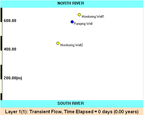
Video: visualization of stream depletion due to pumping; although the analytical solution is derived under specialized assumption, it is often used when the assumptions are not satisfied. Model parameters: Q = 500 GPM; Hydraulic conductivity of the aquifer: 100
ft/day; Aquifer thickness: 100 ft; Effective porosity: 0.2; River stage difference: 25 ft
MAGNET/Modeling Hints:
- Use ‘Synthetic mode’ in MAGNET to create a model domain.
- You may follow the model set-up described in the animation caption above.
- Use line and features as prescribed head boundaries to generate the head difference from the south edge to the north edge of the model.